Access can be used to hold much more than just business data. In this article, David begins a series that looks at the tools you’ll need to work with spatial data stored in Access.
Access, as a database system, is widely used for storing all kinds of data. Traditionally, these include systems like stock control, accounts receivable, and personnel management. An increasing trend is to store geographical data that might be extracted from a plan or map. Over the next three issues of Smart Access, I’ll show you how Access can be used to store and process such data. These principles apply equally well to other applications as well, such as graphics programs, routing systems, or any other spatially based problems.
I’ll start off this series by describing how to represent linear geographical data using the relational model. This includes a detailed breakdown of the most fundamental of all geographical functions — line intersection. In the second article, I’ll describe functions to calculate areas and determine whether a point lies within a given area. Finally, the third article will tie it all together and show how to use these functions in a real-world application.
Unlike the information stored in a more traditional database system, raw geographical data, represented by X,Y coordinates (or Eastings and Northings for larger areas), isn’t always directly interpretable. As a result, it will usually have to undergo significant processing in order to extract meaningful information. For example, you might want to know whether a certain point lies within the area defined by an irregular polygon. This question is often impossible to determine just by a look at the raw data, and you’ll almost certainly have to undergo some form of non-trivial processing before arriving at the correct answer. This enhanced processing requirement is one of the more significant differences between geographical data and traditional data found in an order-processing system.
Understandably, the relatively sophisticated mathematical functions required to process this raw geographical data are missing from Access, as they are from most other programming languages apart from the specialized mathematics packages. So, we’ll have to roll our own. One of the most widely used of these functions is the one that can determine whether two given lines intersect.
If you haven’t written such functions before, you might be mentally questioning the claim that they’re “widely used.” After all, how many situations require you to find out whether two lines intersect? Well, it happens quite a lot! Not only are there the obvious direct uses, such as “at what location does this road cross the county boundary?”, but many of the other geographical functions require the use of the line-intersection function. One perhaps non-intuitive example is, “Does this point lie within a given irregular polygon?” That function would let you create and use irregularly shaped buttons.
But, before we rush into the code, let’s step back a little and consider how we can represent line data in an Access database.
Linear representation
What data do you need to store about a line? A line consists of four numeric values — an X and a Y coordinate for the start of the line, and the same again for the end of the line. Typically, these will contain real numbers and need to be defined as doubles.
Usually, you’re dealing with more than one type of line, such as electricity lines, roads, and political boundaries, so you also need a line type identifier. Often, a simple code will do here.
One snag with this representation is the lack of a suitable primary key candidate. The obvious choice is to use the start point — that is, a composite key of the StartX and StartY fields. However, this can’t be guaranteed to be unique, since other lines might start from the same point. Indeed, you’ll often get lines completely superimposed on each other, thus having identical coordinates at many physical locations. In some applications, the lines might have already been referenced in some way. If so, then you can add this field to the table and use it as the primary key. Failing this, you’ll have to add an AutoNumber field and use that. The layout of the final Lines table might look like Table 1.
Table 1. The simple line table.
| Field Name | Field Type |
| LineID | AutoNumber (or line number if available). |
| LineStartX | Double. |
| LineStartY | Double. |
| LineEndX | Double. |
| LineEndX | Double. |
| LineType | String (or Integer). |
So far, I’ve only discussed single lines with a start/end coordinate. In practice, though, most lines, such as the power, road, and political ones mentioned above, can’t be represented by a single vector. Instead, they’re comprised of a series of linked vectors often referred to (by me at least!) as a “polyline.” These require a slightly more sophisticated treatment. Polylines consist of sets of start/end coordinates where the end coordinate of one section of the line is the same as the start coordinate of the next section. In order to normalize the data, you must remove the redundancy that this creates. You also need a means of associating the different sections of line together — that can most easily be achieved by adding a simple incremental counter field (but not an AutoNumber field) to indicate which segment of the line you’re dealing with. In most instances, you’ll want to use a two-table approach, with the first table consisting of one entry for each line. This table contains the line ID together with any data that refers to the line as a whole — such as the line type, ownership (who owns that pipeline?), and so on. A second table can then be constructed to contain the detailed coordinate data for each line segment. A typical design is shown in Table 2 and Table 3.
Table 2. The Polyline header table.
| Field | Type |
| LineID | AutoNumber (or line number if available). |
| LineType | String (or Integer). |
| ClosedArea | Yes/No. |
| LineOwnership | String (or Integer). |
Table 3. The Polyline detail table.
| Field | Type |
| LineID | As per tblPolyLine. |
| LineSection | Integer. |
| LineX | Double. |
| LineY | Double. |
The primary key for tblPolyline is LineID, as it was for the simple line table. The primary key for tblPolylineDetail is the composite key formed from LineID and LineSection. Although I’ve been talking about lines, the same representation can be used for areas. An area is definable as a polyline whose final end point is the same as its start point. In theory, we could rely on this definition and just test the polyline’s start and end points to determine whether it represented an area rather than a line. In practice, however, the data is unlikely to be clean enough to allow us to use this, so I’ve introduced an additional field (ClosedArea) to indicate whether we’re referring to an area or a line entity.
While on this topic, let me mention that it’s good practice to tidy up the raw data before processing. This includes the removal of duplicated coordinates and making sure that any area entities are closed. In this particular article, you don’t need to make further use of the data representations that I’ve just described. However, I’ll be coming back to them when discussing area calculations in the next article and, again, in the final article, when I’ll describe how these functions can be used in a real-world example.
Code lines
You could just use the four individual coordinates (StartX, StartY, EndX, and EndY) when processing the data. Frequently, though, this results in clumsy coding. A more elegant solution is to create a user-defined line type, there being no intrinsic “line” type in Access. As you’ve seen, a line is defined by a pair of coordinates, one for the start and one for the end of the line, so that you can declare a user-defined line type called LineXY, as shown in the following code:
Type LineXY

    dblStart_X As Double

    dblStart_Y As Double

    dblEnd_X As Double

    dblEnd_Y As Double

End Type
LineXY(0,0,10,10) represents a line that starts at the origin (0,0) and ends at the location (10,10). Okay, that’s got the data defined, so you’re ready to go on to the line intersection function.
To intersect
Please note that this example is in Access 97 (although it could easily be adapted for other versions), and that standard error trapping has been removed for the sake of clarity. Also note that I’m a software developer, not a mathematician or a geographer, so please make allowances for any imprecise geo-mathematical terminology (such as the term geo-mathematical!).
The “Intersect” function in Listing 1 uses the user-defined line type LineXY to pass across the details of the two lines to be tested. The return value from Intersect is a simple Boolean True or False to indicate whether line1 crosses line2 or not. If you also want to return the actual X and Y coordinates of the intersection point, just add a couple of extra Double arguments to the function declaration.
Within this function you’ll be using the mathematical equation for a line, which is Y = M*X + C, where X and Y are coordinates, M is the slope of the line, and C is a constant offset.
The first situation I handle is the special case when two lines are parallel, since there can be no intersection between parallel lines. A line is parallel if it has the same slope as another line, so you need to calculate the slopes of the two lines, or M from our first formula. The formula for M is (Ys – Ye)/(Xs – Xe). You can, therefore, plug in the known values and calculate the slope of the two lines. Note that you have to take into account the special case where the two X coordinates are the same (that is, the line is vertical), which would have you dividing by zero. In this situation, the slope approaches infinity, but I’ve just set it to a very large number. In practice, you might want to treat vertical (and horizontal) lines separately by detecting them at an earlier stage and passing them to modified Intersect functions.
Once you’ve calculated the two slopes, you can com-pare them to see whether they’re the same. Because you’re dealing with real numbers, you can’t do a straight com-parison. Instead, you must test to see whether they’re nearly the same. If the two slope values are almost ident-ical, then the lines are parallel (from a pragmatic point of view, at least), and that means that you can set the return value to indicate that there’s no intersection point and abandon any further processing.
To infinity
Having gotten to this stage, you can now calculate the theoretical intersection point of the two lines. Effectively, this means treating the lines as if they were of infinite length and working out where they would cross (any two non-parallel lines must cross somewhere if they’re extend-ed far enough).
To calculate the theoretical crossing point, you first substitute the previously calculated slope values into the line equations and determine the two constant values C. At the intersection, the X and Y coordinates will be ident-ical for both lines (by definition). The lines’ common X can be calculated as (C2 – C1)/(M1 – M2). With that known, you can now feed the common X coordinate into either of the standard line equations in order to calculate their common Y.
Finally, the InBetween function compares this theoretical intersection point with the coordinates of each line (remember, this intersection point is based on the assumption that the lines were infinitely long). InBetween determines whether the intersection point lies outside of the range of either line because, if it does, there’s no intersection. Voila! You have your answer.
The only additional points to consider are the special cases for horizontal lines, and when the lines touch but don’t actually cross. This is handled in the InBetween function by the addition of dblSmidgin (just a small number) into the comparison. dblSmidgin compensates for the problems of comparing two real numbers for equality. If, as suggested, you treat vertical and horizontal lines as special cases with slightly different processing, you can probably remove dblSmidgin from the standard routine. All the code can be found in Listing 1.
Listing 1. The code to determine whether the two lines intersect.
Public Function Intersect(ByRef Line1 As LineXY, _

 ByRef Line2 As LineXY) As Boolean

 ' Copyright 1997, Aldex Software

 ' Equation for a line is Y = M*X + C

 ' NB calls the function InBetween

 ' Author D.P.Saville, Aldex Software,

 ' dps@aldex.co.uk, http://www.aldex.co.uk/

 ' July 1997


Dim dblSlopeLine1 As Double, dblSlopeLine2 As Double

Dim dblCLine1 As Double, dblCLine2 As Double

Dim dblX As Double, dblY As Double


' First, calculate the slope of the lines

If Abs(Line1.dblStart_X - Line1.dblEnd_X) _

 < 0.0000000001 Then 'Line is vertical

  dblSlopeLine1 = 1000000000000# ' close to infinity

Else

  dblSlopeLine1 = _

  (Line1.dblEnd_Y - Line1.dblStart_Y) _

  / (Line1.dblEnd_X - Line1.dblStart_X)

End If


If Abs(Line2.dblStart_X - Line2.dblEnd_X) _

  < 0.0000000001 Then  'Line is vertical

  dblSlopeLine2 = 1000000000000# ' close to infinity

Else

  dblSlopeLine2 = _

  (Line2.dblEnd_Y - Line2.dblStart_Y) _

  / (Line2.dblEnd_X - Line2.dblStart_X)

End If


If Abs(dblSlopeLine2 - dblSlopeLine1) _

  < 0.0000000001 Then

  ' Lines are parallel

  Intersect = False

  Exit Function

End If


' Find where the lines WOULD intersect

' if they were of infinite length.


' Pull out the Constant value from each line

dblCLine1 = Line1.dblEnd_Y - _

  (dblSlopeLine1 * Line1.dblEnd_X)

dblCLine2 = Line2.dblEnd_Y - _

  (dblSlopeLine2 * Line2.dblEnd_X)


' Feed this Constant and Slope

' into the equations to find

' the potential intersect point.

dblX = (dblCLine2 - dblCLine1) _

 / (dblSlopeLine1 - dblSlopeLine2)

dblY = (dblSlopeLine1 * dblX) + dblCLine1


' test to see if the intersect actually happens within

' the start and end of the two lines.

If InBtw(dblX, Line1.dblStart_X, Line1.dblEnd_X) And _

 InBtw(dblX, Line2.dblStart_X, Line2.dblEnd_X) And _

 InBtw(dblY, Line1.dblStart_Y, Line1.dblEnd_Y) And _

 InBtw(dblY, Line2.dblStart_Y, Line2.dblEnd_Y) Then

    Intersect = True

Else

    Intersect = False

End If


End Function


Private Function InBtw(pdbl, pdblStart, pdblEnd) _

  As Boolean

' Used by the Intersect() to test if intersect point

' pdbl lies between pdblStart to pdblEnd.

' dblSmidgin is used to account for horizontal lines,

' which may need altering, depending upon your data.

Const dblSmidgin As Double = 0.01


If pdbl >= (pdblStart - dblSmidgin) And _

  pdbl <= (pdblEnd + dblSmidgin) Then

    InBetween = True

    Exit Function

ElseIf pdbl <= (pdblStart + dblSmidgin) And _

       pdbl >= (pdblEnd - dblSmidgin) Then

        InBetween = True

        Exit Function

Else

    InBetween = False

End If

End Function
To reality
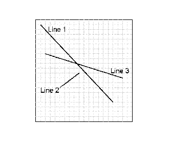
Figure 1
Now that I’ve finished walking through the actual Intersect function, you’d probably like a smattering of real code to show how you might call the function. Here’s the code to compare the three lines shown in Figure 1:
 Dim Line1 As LineXY

    Dim Line2 As LineXY

  Dim Line3 As LineXY


    Line1.dblStart_X = 1

    Line1.dblStart_Y = 19

    Line1.dblEnd_X = 16

    Line1.dblEnd_Y = 4


    Line2.dblStart_X = 5

    Line2.dblStart_Y = 7

    Line2.dblEnd_X = 9

    Line2.dblEnd_Y = 10


    Line3.dblStart_X = 2

    Line3.dblStart_Y = 14

    Line3.dblEnd_X = 18

    Line3.dblEnd_Y =9


    Debug.Print "Intersect=" & Intersect(Line1, Line2)

    Debug.Print "Intersect=" & Intersect(Line1, Line3)
The intersect for line 1 (1,19)-(16,4) and line 2 (5,7)-(9,10) should be False, with the theoretical intersect point occurring at (9.571, 10.428). The intersect point of line 1 with line 3 (2,14)-(18,9) should be True, with an intersect at (7.818,12.181).
Although these routines have all been tested, the reality is that you must test them again with your own data before using them. This is especially true because we’re dealing with real-world data containing real numbers, not integers (as is evident from the approximations and comparisons the routines use). Furthermore, some applications will be dealing in relatively small X/Y coordinates, whereas others might be using values of literally global extent.
Horizontal and vertical lines create their own special problems. In practice, I prefer to extract these and treat them as special cases with modified versions of the Intersect algorithm (it improves performance as well), rather than using the same algorithm for all. So, as I said, please test this thoroughly using your own data.
While this article has assumed geographical data, these routines will, in fact, work with any X, Y co-ordinates — even ones on your computer screen. These functions (and the ones in the next article) give you the ability to create graphical front ends to your Access application — even to create image maps like the ones used on the World Wide Web. Like the horizon, the possibilities are endless.
See Accessing Spatial Data, Part 2 Accessing Spatial Data, Part 3