You should never calculate the average value of anything without also calculating the median value. Chris Weber explains why and gives you a clean, step-by-step method for deriving the median value from any numeric series. Unlike other published methods, Chris’ method uses no temporary tables or custom functions–all you need is a single query.
It bothers me that we’re inundated through the media with statistics about the average this and the average that, and people accept these numbers as meaningful. If you need to determine a “typical value,” shouldn’t you just add everything up and divide by the number of items you added up (in other words, calculate an average)? The only problem is that if you need a typical value, you might not really need an average–you might need a median. Average, median: What’s the difference? And, more importantly, do you even care? The problem is that the average anything is only meaningful if there are a significant number of observations, and the distribution of numbers being examined has a somewhat even or continuous distribution. In many cases, the average is actually a lie (or, at best, a misleading truth). Given the limitations that I’ve listed, you might think that an average is never the right answer.
Consider the following two datasets reflecting taxation in thousands of dollars for 11 buildings on the east and west sides of a city block (Table 1). The average taxation (that is, the “typical value” calculated by adding up the numbers and dividing by the number of items) for both groups is $7,640.00.
Table 1. The tax burden on two sides of a city block.
| East side | West side | |
| Unit 1 | 4,260 | 2,220 |
| Unit 2 | 5,260 | 3,250 |
| Unit 3 | 6,280 | 4,820 |
| Unit 4 | 6,950 | 5,560 |
| Unit 5 | 7,490 | 6,660 |
| Unit 6 | 7,780 | 6,780 |
| Unit 7 | 8,240 | 6,850 |
| Unit 8 | 8,330 | 7,450 |
| Unit 9 | 9,250 | 7,590 |
| Unit 10 | 9,960 | 7,610 |
| Unit 11 | 10,250 | 25,230 |
| Average | 7,640 | 7,640 |
However, if you graph the results (see Figure 1), you can see that there’s an outlier on the west side (perhaps this is a new high-rise building). The presence of this extraordinarily high tax source completely skews the mean average for the west side of the block. If you compare the tax burden for the individual buildings on the east side and the west side, you can see that the east side buildings typically pay much more in taxes than the west side. If you were deciding which side of the block you were going to build on, you’d want to build on the west side where you could pay less in taxes (all other things being equal). However, an average value conceals this information by making the two sides look alike: The “typical value” calculating for the west side isn’t really typical at all.
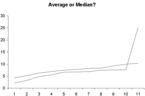
Figure 1
On the other hand, you could calculate the median value and use that instead of the average value. If a set of observations is arranged in ascending or descending order, the median is the middle value when the number of observations is odd, or the average of the two middle values when the number of observations is even. In Table 1, I’ve already sorted the tax burdens for the two blocks into ascending order, so it’s easy to see the median value of the two sides of the block. If you look at the median (row 6 for this odd number of observations) instead of their average, you can see that the majority of buildings on the west side of the street are taxed at a significantly lower rate ($6,780.00) than the east side ($7,780.00). That apartment building was inflating the typical value for the tax rate for buildings on the west side.
If you want to make sure that your “typical value” really is typical, you should calculate your average and your median value and only consider the values “typical” when the two are very close. You’re probably aware that Access provides built-in support for calculating mean average in totals queries by using the Avg aggregate SQL statement, and in code with the DAvg() domain function. Wouldn’t it be nice to have built-in support for the median as well? Sorry, no such luck. You could buy a third-party statistics add-in package, but as you’ll see, it’s really not so difficult to solve this problem with relatively simple queries.
Calculating the median
Over the years, I’ve read numerous solutions to finding the median in a dataset. These solutions appear from time to time in Smart Access and other Access and SQL Server journals. Microsoft has published several Knowledge Base articles (including 95918 “How to Use Code to Derive a Statistical Median”), but these, like many articles covering the topic, are procedural in nature. By “procedural,” I mean that these methods depend heavily on writing code that will execute in the proper order (though they may use calculations within queries or recordsets in VBA). These methods don’t leverage our access to the Jet database engine and the version of SQL at our disposal. These solutions also often involve temporary tables and, sometimes, the process is difficult to follow.
If you were to manually derive the median of a dataset, you’d first order the data in ascending or descending order. You’d then find the middle value, whether it be the center value in an odd number of rows or the mean average of the two innermost values in an even number of rows. In any attempt to solve the median riddle, the trick is to uncover a quick way to find those middle values.
I’ll start with the data in Table 2 with any number of rows from which I need to derive the median. In my example, I’ve chosen to use an even 10 values just to make my test more interesting.
Table 2. A set of 10 values to calculate a median.
| Data |
| 35 |
| 73 |
| 74 |
| 86 |
| 86 |
| 87 |
| 92 |
| 94 |
| 95 |
| 99 |
I realized that I could get at the middle value(s) of any dataset by executing two TOP values queries and focusing on the last value in each result set. I’ll call these two queries Top50PercentAsc_Step1a and Top50PercentDesc_Step1b. The first query takes the top 50 percent of the entries with the dataset sorted in ascending order (the default); the second query takes the top 50 percent of the entries but this time with the dataset sorted in descending order:
SELECT TOP 50 PERCENT Table1.data AS LowerMedian

FROM Table1

ORDER BY Table1.data;

SELECT TOP 50 PERCENT Table1.data AS UpperMedian

FROM Table1

ORDER BY Table1.data DESC;
The results of the two queries can be seen in Table 3. If any ties had been encountered at the center of the dataset, both queries would return the same value in the last position.
Table 3. The results of the queries Top50PercentAsc_Step1a and Top50PercentDesc_Step1b.
| LowerMedian | UpperMedian |
| 35 | 99 |
| 73 | 95 |
| 74 | 94 |
| 86 | 92 |
| 86 | 87 |
Now, taking the average of the last value in Top50PercentAsc_Step1a and Top50PercentDesc_Step1a should give me my median answer. So my next step was to pull out those two numbers by using the Max function on the results of the Top50PercentAsc_Step1a query and the Min function on the results of the Top50PercentDesc_Step1b. Here are the two queries, with the results shown in Table 4:
SELECT Max(Top50PercentAsc_Step1a.LowerMedian)

                              AS MaxOfLowerMedian

FROM Top50PercentAsc_Step1a;

SELECT Min(Top50PercentDesc_Step1b.UpperMedian)

                              AS MinOfUpperMedian

FROM Top50PercentDesc_Step1b;
Table 4. The lowest and highest numbers from Top50PercentAsc_Step1a and Top50PercentDesc_Step1a.
| MinOfUpperMedian | MaxOfLowerMedian |
| 87 | 86 |
My last step is to average these two “TOP” values into a single query (called qryMedianFromNestedQueries) to get the median value. This query does that, and the results are shown in Table 5:
SELECT ([MinOfUpperMedian]+[MaxOfLowerMedian])/2 AS Median

FROM Top50PercentDesc_Step2b, Top50PercentAsc_Step2a;
Table 5. The median of the original dataset.
| Median |
| 86.5 |
If there had been an odd number of values, then the two input queries to this process would have returned the same value and this query would be calculating the average of two identical numbers (a calculation that, I imagine, goes very quickly).
Simplifying
As simple as this method is, it bothers me to have to build and nest five queries to get the result. It’s not that building the queries is difficult. I just don’t like keeping all of those objects in my database for a single output. To reduce that number, I’m going to show you a single query approach inspired by an example in Doug Steele’s “Access Answers” column in the February 2005 issue. And, as Doug said, this approach works with Jet 4.0 (Access 2000 and newer) but not with Jet 3.6 (Access 97).
I’m going to rework my example from the inside out. First, note that the results from Table 4 could be combined into a single table by using a Union query (in a Union query, if you have different names for the fields in the queries being Unioned, then the names for the fields are taken from the first query in the Union). This reduces my original solution to four queries (the result of this query is shown in Table 6):
SELECT Max(Top50PercentAsc_Step1a.LowerMedian)

                                  AS MaxOfLowerMedian

FROM Top50PercentAsc_Step1a;

   UNION

SELECT Min(Top50PercentDesc_Step1b.UpperMedian)

                                  AS MinOfUpperMedian

FROM Top50PercentDesc_Step1b;
Table 6. A single Union result of two queries.
| MaxOfLowerMedian |
| 86 |
| 87 |
If I take the average of the result of my Union query, I have my answer. I can compute this average with a single statement by using this new Union query as the input to the query that calculated the average. Now my solution is down to just three queries:
SELECT Avg([MaxOfLowerMedian]) AS Median

FROM

  [

   SELECT Max(Top50PercentAsc_Step1a.LowerMedian)

                                AS MaxOfLowerMedian

   FROM Top50PercentAsc_Step1a

      UNION

   SELECT Min(Top50PercentDesc_Step1b.UpperMedian)

                                AS MinOfUpperMedian

   FROM Top50PercentDesc_Step1b

  ]. AS UnionOfResults
In the first line, I used the SQL Avg function with the MaxofLowerMedian field name, the name selected by the Union query for its output field. Secondly, in the SQL statement where I’ve replaced the query name that I used originally with a Union query, I’ve put that Union statement inside brackets and assigned it an alias (UnionOfResults). Don’t ignore that period after the last bracket and before the AS statement. That period indicates to Jet that the bracketed statement is ended and Jet shouldn’t to expect a field name to follow the bracket. Also, I was sure to remove any semicolons from my now-nested queries (Jet interprets the semicolon as an end-of-SQL marker).
Following this same pattern, you may have guessed that the two innermost queries, Top50PercentAsc_Step1a and Top50PercentDesc_Step1b, can also be nested within my statement. This time, I’ve used parentheses and haven’t had to use the period before the alias name. Just as in a lengthy algebraic statement, you may want to alternate brackets and parentheses to make the statement more readable. I’ve also assigned aliases to the output of the Min and Max aggregations to make the Union output consistent:
SELECT Avg([Result]) AS Median

FROM

 [

   SELECT Max(Top50PercentAsc.LowerMedian) AS Result

   FROM

        (SELECT TOP 50 PERCENT Table1.data

                                        AS LowerMedian

         FROM Table1

         ORDER BY Table1.data ASC) AS Top50PercentAsc

     UNION

   SELECT Min(Top50PercentDesc.UpperMedian) AS Result

   FROM

        (SELECT TOP 50 PERCENT Table1.data

                                        AS UpperMedian

         FROM Table1

         ORDER BY Table1.data DESC) AS Top50PercentDesc

 ]. AS UnionOfResults
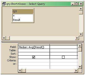
My solution is now a single query, albeit one that you may want to construct using the earlier examples (and then throw the earlier queries away once you’ve built the single query). You could continue, and make your statement shorter by shortening the alias names to mere placeholders like Q1, Q2, Q3 as this example does (whether the loss of descriptive names makes the shorter version more or less readable is up to you):
SELECT Avg([R1]) AS Median

FROM

  [

   SELECT Max(Q1.R2) AS R1

   FROM

       (SELECT TOP 50 PERCENT Table1.data AS R2

        FROM Table1

        ORDER BY Table1.data ASC) AS Q1

    UNION

   SELECT Min(Q2.R2) AS R1

   FROM

       (SELECT TOP 50 PERCENT Table1.data AS R2

        FROM Table1

        ORDER BY Table1.data DESC) AS Q2

  ].

  AS Q3;
If you view this sort of nested SQL in Design View, the innermost queries are buried within the second-to-last nesting, which is displayed in the table pane (see Figure 2). As a result, Design View probably isn’t useful for designing these kinds of statements, and is certainly useless for understanding what’s happening. This is just one of those times when the ability to read SQL is necessary.
Figure 2
Using the query in Access 97
I stated earlier that this nested SQL won’t work in Access 97. That statement isn’t completely true. If you convert a database with a nested query like this from Access 20** back to Access 97, the query will work. However, if you attempt to alter the query in any way, it will cease to function and return “Syntax error in FROM clause” when you run it. Even just cutting and re-pasting the SQL into the Query Editor will break the query. Presumably, the compiled version of the query is successfully migrated from Access 20** to Access 97. However, if Access 97 is forced to reinterpret the query because you’ve changed the text, the query is beyond the abilities of Access 97 to handle.
I’ve included all my examples in the sample database that accompanies this article. Table1 in the database is loaded with the sample data from this article. I’ve also included a public module with a procedure that lets you load the table with any number of randomly generated values between 1 and 101. To run this code, open the module, click anywhere in the procedure, and press F5. You’ll be prompted for the number of values you’d like. To see the median for that data in a table, just run qryMedianAllInOne or qryMedianFromNestedQueries. You can check that you’ve got the right answer by checking the last values in Top50PercentAsc_Step1a and Top50PercentDesc_Step1b to see that my query works as advertised.
Oh–and when you read that the average American home sells for this or the average worker is paid that, don’t believe it. Ask for the median.
Other Pages that You Might Like to Read
An Average Column: I Mean, What Mode is Your Median
Top Values, Hierarchical Lists, and Almost Equivalent Strings
Numerical Sequence